Here’s a step-by-step tutorial with easy steps to follow.
1. Identify the Columns for the Given Date and Number of Days to be Added
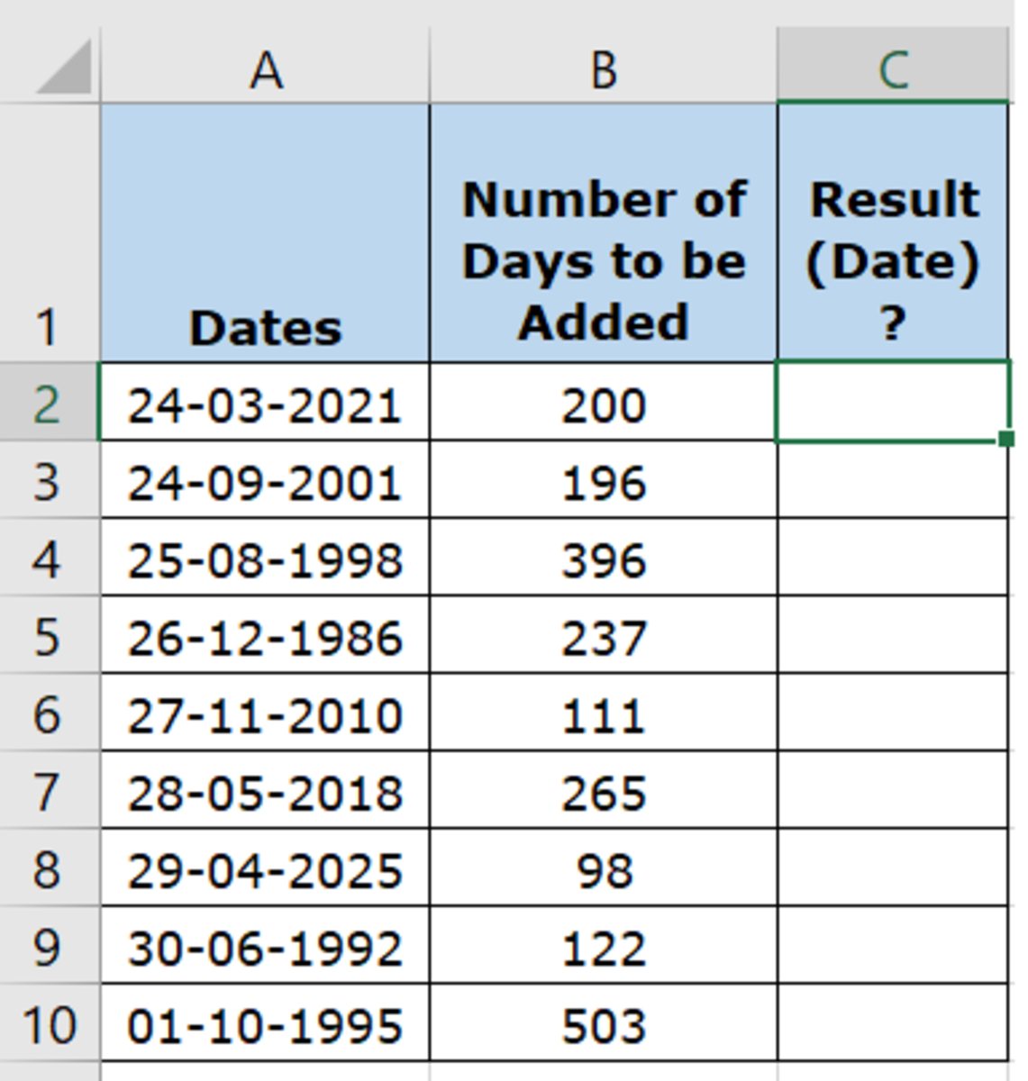
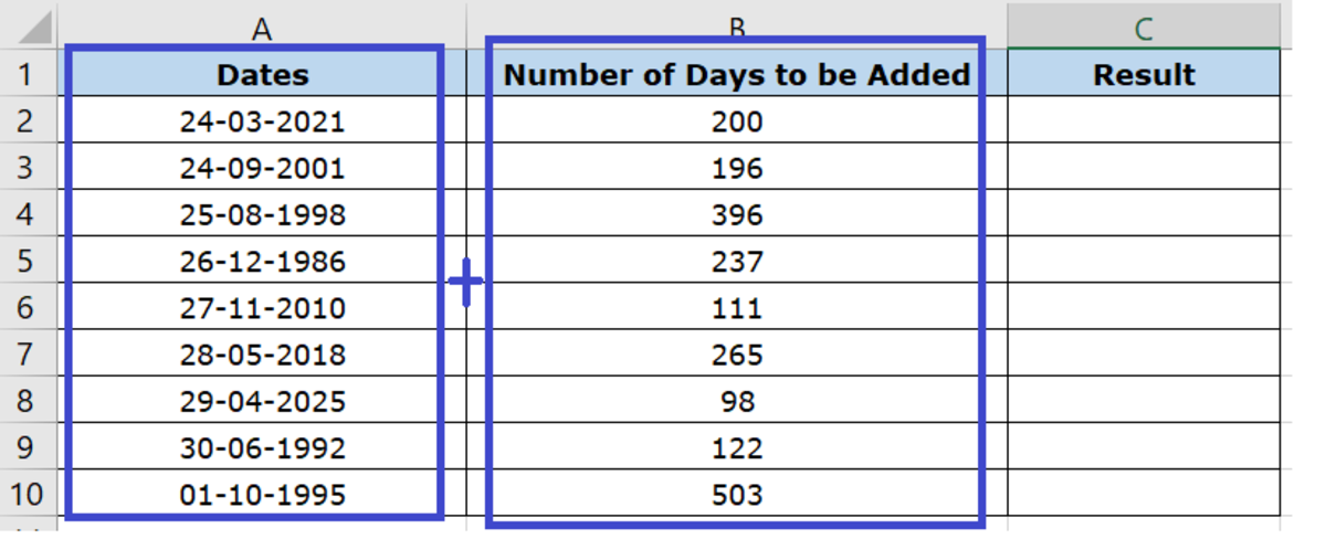
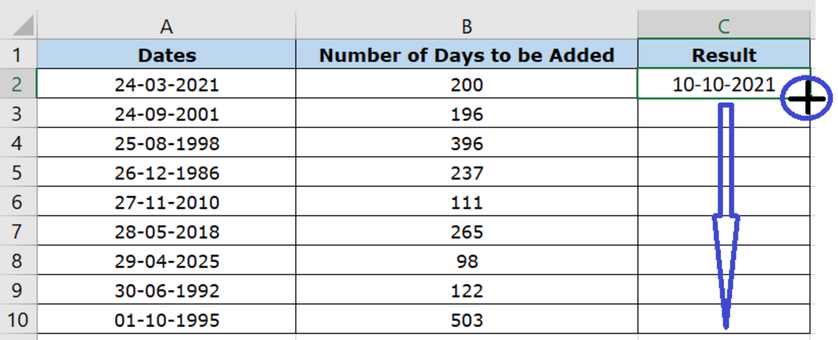
Let us assume we have a list of dates in a Microsoft Excel Worksheet, and we would like to add a certain number of days to these dates and get the result in date format. Here’s the sample data we are going to use to demonstrate how to do this. In our table here, we have a list of dates in the (DD-MM-YYYY) format and a number of days to be added to these dates in number format. We are going to use Microsoft Excel Formulas to automatically add the number of days to the dates and get the result in date format. So, in this case, the date column to be used would be Column A, that is holding the Date values. And the number of days are stored in Column B.
2. Apply the Formula in the Cell Where the Resultant Date Should Appear
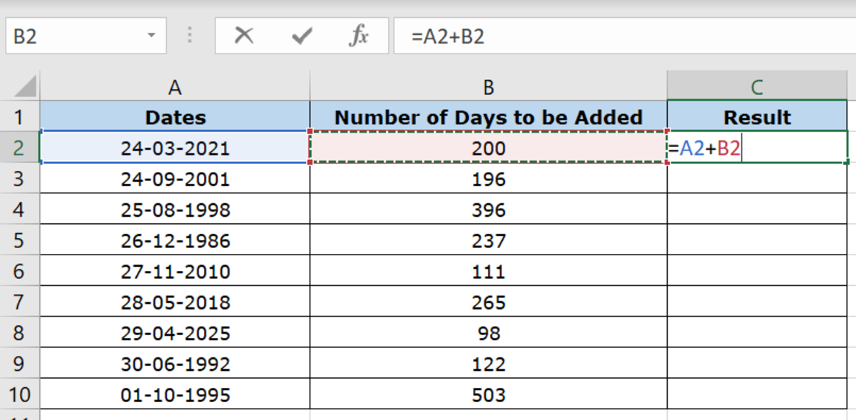
Formula to be entered in cell: C2 (That’s where the Resultant Date should appear after adding the number of days (B2) to the given date (A2)) Formula to be used: =<Column ID 1>+<Column ID 2> The Formula adds the number of days in Column B to the Date in Column A and calculates the result in date format. Keep in mind,
Column ID1 is the cell that holds the Date value. In this case, it is A2. Column ID2 is the cell that holds the number of days to be added to the date value. In this case, it is B2. So our formula becomes: =A2+B2
3. Copy the Formula to the Remaining Cells
You could either copy and paste the formula in the remaining cells, or you could drag the plus sign at the bottom right corner of the cell so that the formula gets copied to the remaining cells.
And Done!
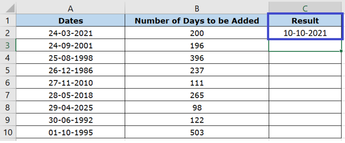
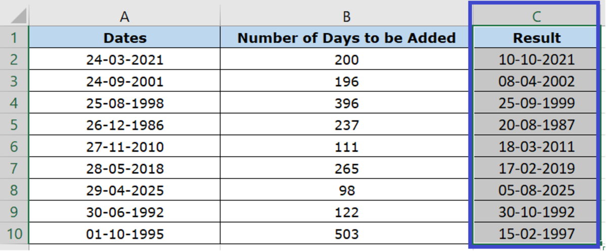
Once the formula is copied to the other cells, it automatically adds the number of days in Column B to the dates in Column A, and the resultant value appears in Column C in Date Format. This content is accurate and true to the best of the author’s knowledge and is not meant to substitute for formal and individualized advice from a qualified professional. © 2021 Petite Hubpages Fanatic
